Lesson 09 - Multidimensional Arrays & Sorting

Multidimensional Arrays

Multidimensional arrays are just like the basic arrays we learned about last lesson, except they can hold values in more than one dimension. There are a few ways of thinking about the layout—the simplest is probably to think of a two dimensional array as simply an array of arrays. That's how it works at a low level. However, you can also visualize a two dimensional array, again for example, as a two-dimensional grid of values rather than simply a one-dimensional line of them. Either way can extend to more dimensions than two—for example, a three dimensional array is simply an array of arrays of arrays, or a three dimensional cube of values. It’s not too complex if you think about it.

However, the spatial visualization doesn’t work so well with arrays of greater than three dimensions.

Using Multidimensional Arrays

Declaring a multidimensional array is almost exactly the same as a one-dimensional array: you just add the sizes of each dimension you want onto the end.

array2D[10][10];

Declares an array with dimensions 10 by 10.

array4D[10][10][10][10];

Declares a four dimensional array with dimensions 10 by 10 by 10 by 10.

Using multidimensional arrays is also almost exactly the same as with one-dimensional arrays: you reference each value by specifying the index. Except now you must specify the index in each of the dimensions.

Remember that I mentioned that 2D arrays are really just arrays of arrays at a low level? Well, this comes into play here. For example, if you only specify the first dimensional index in a 2D array, you will get the entire array that goes with that first index. Likewise, if you only specified the first index in a 3D array, you will receive the corresponding 2D array, and so on.

array2D[4][4];

Accesses the element at location 4, 4.

array4D[0][0][0];

Accesses the entire one dimensional array stored at the location 0,0,0 in the 4D array.

Passing multidimensional arrays to functions is, yet again, almost exactly the same as one dimensional arrays. Except with one catch—you have to specify the length of every dimension except the first. This means that if you want to pass a 2D array into a function, you don’t have to know how the size of the first dimension, but you have to know the size of the second dimension. This is because all data is stored in memory linearly. For example, in a 2D array, the first data represents the array at index 0. Hence, the computer must know how long this array (the second dimension, see?) is in order to tell when it has reached the next index in the first dimension.

However, all this can be largely disregarded when using pointers and dynamic memory. See lesson 10 and 11.

Finally, again, to pass an array into a function, simply pass the name with no brackets at all.

void func(int[][10]);

void func(int array[][10]) {
	// do stuff
}

This declares and implements a function that will take an integer array with any first dimension size, but only a second dimension size of 10.

int array2D[5][10];
func(array);

This calls the function with the 2D array “array2D.”

One last remark. Again as with one-dimensional arrays, you’re most often going to want to manipulate multidimensional arrays with loops. Nested loops are particularly useful for this purpose, as you can simply write "array[i][j]" and not have to worry about any fancy math.

for(int i = 0; i < 10; i++) {
	for(int j = 0; j < 10; j++) {
		array2D[i][j] = 0;
	}
}

This sets all values in a 2D array with dimensions 10 by 10 to 0. In this example, the program will first loop though all 10 values in array2D[0], then those in array2D[1], and so on, until all 100 values have been passed over.

Arrays of C-Strings

An array of c-style strings is technically just a two-dimensional array of characters. However, you can still logically think of it as simply an array of c-string values, as each element in an array of c-strings is it's own c-string with all the properties you've learned. This should illustrate the fact that if you specify only the first index in a 2D array, you get the entire 1D array at that index. You select the first index in a 2D character array, and receive a 1D character array—a c-string.

char cstringArr[10][50];

This declares an array of 10 c-strings, each with a size of 50 characters.

for(int i = 0; i < 10; i++) {
	cout << cstringArr[i] << endl;
}

This will loop though the array of 10 c-strings and output each one. Remember that you can use each element of the first dimension of the c-string array as a c-string.

Sorting

In the previous few lessons I’ve mentioned ways of sorting arrays. Sorting is simply ordering values of an array in a particular sequence—for example, lowest to highest or vice versa. We’ll go over a few different methods of sorting, otherwise known as sorting algorithms.

Bubble Sort

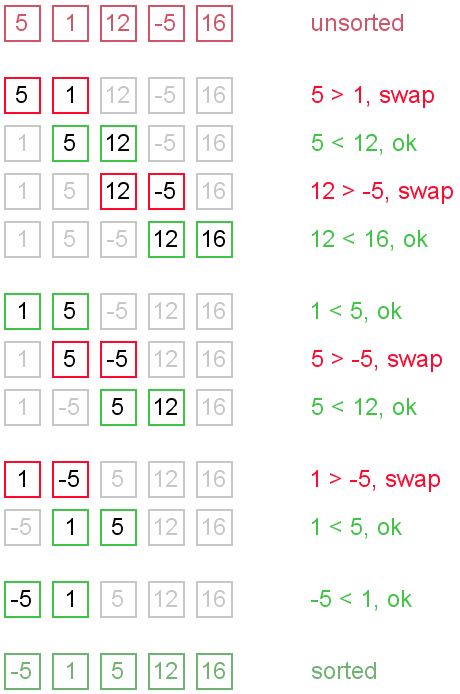
The bubble sort is the simplest of sorts to write code for, but it is also one of the most inefficient. Essentially, the algorithm will loop through the array, and whenever it finds a pair of values where one is larger than the next, it will swap the values and keep going. This means that higher values will “bubble up” in the array until they find their correct places. Then, it will go back to the beginning and do the same thing again, and again, until the entire array is sorted.

Selection Sort

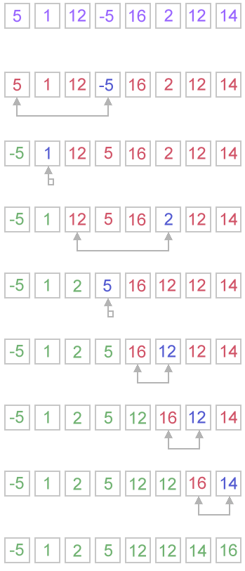
The selection sort is more efficient than the bubble sort and slightly easier to understand, but is a bit more complicated to implement. The selection sort algorithm simply finds the lowest value in the array, puts it in the first spot, finds the next lowest value in the array, puts it in the second spot, and so on. To do this, the algorithm first finds the lowest value in the entire array and swaps it with the first value in the array. Then, it does the same thing, except it starts searching for the lowest value beginning with the second element. When the algorithm finds it, it puts it in the second slot. Finally, it starts searching from the third value, and so on.

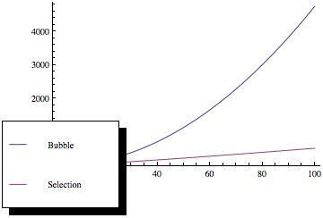
Because the selection sort only has to iterate over the array once for each element, it quickly becomes much less computationally intensive compared to a bubble sort. In the bubble sort, the number of iterations can be much, much higher than the number of elements. In fact, the graph of computation required by your computer compared to the array size looks something like this:

Quicksort

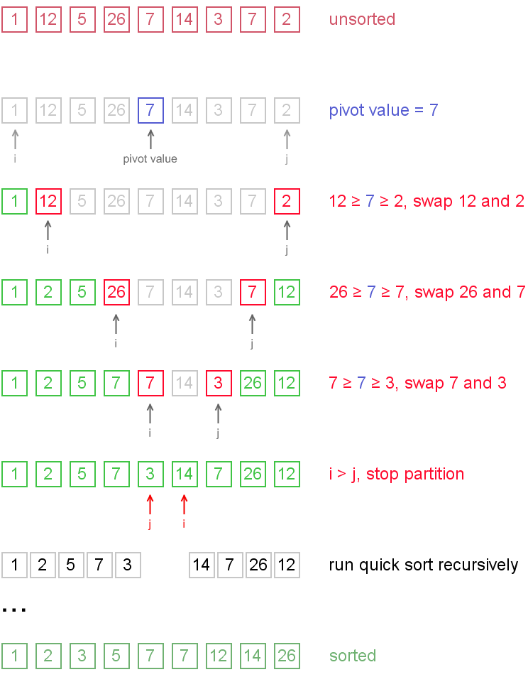
The last sorting algorithm we’ll be covering is the quicksort algorithm, which is the most efficient of the three we’ve seen, but also the most complicated to implement. For this reason, we’ll just be going over the concept (an implementation is provided in the example program). Essentially, the quicksort algorithm sorts the array into two parts (usually called "partitions"). The first partition holds all the lowest values, and the second holds all the highest values. Note that the partitions themselves are not necessarily sorted. Then, the algorithm does the same operation on each partition, so the lower and higher values are split into partitions within both the first and second partition. Now there are four partitions. This process is repeated until each partition size is just one element, hence the array has been sorted.

The visualization should be very useful in understanding this sort.

Other Sorting Algorithms

We’ve only gone over three of many different types of sorting algorithms. If you’d like to learn more, some other types are:

Insertion Sort

the selection sort, but a bit better.

Modified Bubble Sort

the bubble sort, but a bit better.

Exchange Sort

similar to the bubble sort, but compares elements to the first value.

Shell Sort

similar to the bubble sort, but compares elements that are a certain distance away from each other.

Heap Sort

similar to the selection sort, but uses a heap data structure for storage.

Merge Sort

similar to quicksort, but combines sorted arrays (partitions) and can be used effectively with linked lists.