Exploring Neural Graphics Primitives
Neural fields have quickly become an interesting and useful application of machine learning to computer graphics. The fundamental idea is quite straightforward: we can use neural models to represent all sorts of digital signals, including images, light fields, signed distance functions, and volumes.
Neural Networks
This post assumes a basic knowledge of neural networks, but let’s briefly recap how they work.
A network with $$n$$ inputs and $$m$$ outputs approximates a function from $$\mathbb{R}^n \mapsto \mathbb{R}^m$$ by feeding its input through a sequence of layers. The simplest type of layer is a fully-connected layer, which encodes an affine transform: $$x \mapsto Ax + b$$, where $$A$$ is the weight matrix and $$b$$ is the bias vector. Layers other than the first (input) and last (output) are considered hidden layers, and can have arbitrary dimension. Each hidden layer is followed by applying a non-linear function $$x \mapsto f(x)$$, known as the activation. This additional function enables the network to encode non-linear behavior.
For example, a network from $$\mathbb{R}^3 \mapsto \mathbb{R}^3$$, including two hidden layers of dimensions 5 and 4, can be visualized as follows. The connections between nodes represent weight matrix entries:

Or equivalently in symbols (with dimensions):
This network has $$5\cdot3 + 5 + 4\cdot5 + 4 + 3\cdot4 + 3 = 59$$ parameters that define its weight matrices and bias vectors. The process of training finds values for these parameters such that the network approximates another function $$g(x)$$. Suitable parameters are typically found via stochastic gradient descent. Training requires a loss function measuring how much $$\text{NN}(x)$$ differs from $$g(x)$$ for all $$x$$ in a training set.
In practice, we might not know $$g$$: given a large number of input-output pairs (e.g. images and their descriptions), we simply perform training and hope that the network will faithfully approximate $$g$$ for inputs outside of the training set, too.
We’ve only described the most basic kind of neural network: there’s a whole world of possibilities for new layers, activations, loss functions, optimization algorithms, and training paradigms. However, the fundamentals will suffice for this post.
Compression
When generalization is the goal, neural networks are typically under-constrained: they include far more parameters than strictly necessary to encode a function mapping the training set to its corresponding results. Through regularization, the training process hopes to use these ’extra’ degrees of freedom to approximate the behavior of $$g$$ outside the training set. However, insufficient regularization makes the network vulnerable to over-fitting—it may become extremely accurate on the training set, yet unable to handle new inputs. For this reason, researchers always evaluate neural networks on a test set of known data points that are excluded from the training process.
However, in this post we’re actually going to optimize for over-fitting! Instead of approximating $$g$$ on new inputs, we will only care about reproducing the right results on the training set. This approach allows us to use over-constrained networks for (lossy) data compression.
Let’s say we have some data we want to compress into a neural network. If we can parameterize the input by assigning each value a unique identifier, that gives us a training set. For example, we could parameterize a list of numbers by their index:
…and train a network to associate the index $$n$$ with the value $$a[n]$$. To do so, we can simply define a loss function that measures the squared error of the result: $$(\text{NN}(n) - a[n])^2$$. We only care that the network produces $$a[n]$$ for $$n$$ in 0 to 6, so we want to “over-fit” as much as possible.
But, where’s the compression? If we make the network itself smaller than the data set—while being able to reproduce it—we can consider the network to be a compressed encoding of the data. For example, consider this photo of a numbat:
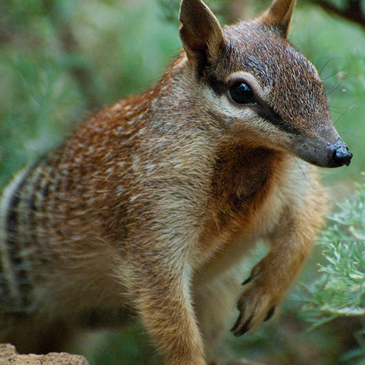 Perth Zoo
The image consists of 512x512 pixels with three channels (r,g,b) each. Hence, we could naively say it contains 786,432 parameters. If a network with fewer parameters can reproduce it, the network itself can be considered a compressed version of the image. More rigorously, each pixel can be encoded in 3 bytes of data, so we’d want to be able to store the network in fewer than 768 kilobytes—but reasoning about size on-disk would require getting into the weeds of mixed precision networks, so let’s only consider parameter count for now.
A Basic Network
Let’s train a network to encode the numbat.
To create the data set, we will associate each pixel with its corresponding $$x,y$$ coordinate. That means our training set will consist of 262,144 examples of the form $$(x,y) \mapsto (r,g,b)$$. Before training, we’ll normalize the values such that $$x,y \in [-1,1]$$ and $$r,g,b \in [0,1]$$.
Clearly, our network will need to be a function from $$\mathbb{R}^2 \mapsto \mathbb{R}^3$$, i.e. have two inputs and three outputs. Just going off intuition, we might include three hidden layers of dimension 128. This architecture will only have 33,795 parameters—far fewer than the image itself.
Our activation function will be the standard non-linearity ReLU (rectified linear unit). Note that we only want to apply the activation after each hidden layer: we don’t want to clip our inputs or outputs by making them positive.

Finally, our loss function will be the mean squared error between the network output and the expected color:
Now, let’s train. We’ll do 100 passes over the full data set (100 epochs) with a batch size of 1024. After training, we’ll need some way to evaluate how well the network encoded our image. Hopefully, the network will now return the proper color given a pixel coordinate, so we can re-generate our image by simply evaluating the network at each pixel coordinate in the training set and normalizing the results.
And, what do we get? After a bit of hyperparameter tweaking (learning rate, optimization schedule, epochs), we get…
| Epochs: 100 |
Well, that sort of worked—you can see the numbat taking shape. But unfortunately, by epoch 100 our loss isn’t consistently decreasing: more training won’t make the result significantly better.
Activations
So far, we’ve only used the ReLU activation function. Taking a look at the output image, we see a lot of lines: various activations jump from zero to positive across these boundaries. There’s nothing fundamentally wrong with that—given a suitably large network, we could still represent the exact image. However, it’s difficult to recover high-frequency detail by summing functions clipped at zero.
Sigmoids
Because we know the network should always return values in $$[0,1]$$, one easy improvement is adding a sigmoid activation to the output layer. Instead of teaching the network to directly output an intensity in $$[0,1]$$, this will allow the network to compute values in $$[-\infty,\infty]$$ that are deterministically mapped to a color in $$[0,1]$$. We’ll apply the logistic function:

For all future experiments, we’ll use this function as an output layer activation. Re-training the ReLU network:
| Epochs: 100 |
The result looks significantly better, but it’s still got a lot of line-like artifacts. What if we just use the sigmoid activation for the other hidden layers, too? Re-training again…
| Epochs: 100 |
That made it worse. The important observation here is that changing the activation function can have a significant effect on reproduction quality. Several papers have been published comparing different activation functions in this context, so let’s try some of those.
Sinusoids
Implicit Neural Representations with Periodic Activation Functions
This paper explores the usage of periodic functions (i.e. $$\sin,\cos$$) as activations, finding them well suited for representing signals like images, audio, video, and distance fields. In particular, the authors note that the derivative of a sinusoidal network is also a sinusoidal network. This observation allows them to fit differential constraints in situations where ReLU and TanH-based models entirely fail to converge.
The proposed form of periodic activations is simply $$f(x) = \sin(\omega_0x)$$, where $$\omega_0$$ is a hyperparameter. Increasing $$\omega_0$$ should allow the network to encode higher frequency signals.
Let’s try changing our activations to $$f(x) = \sin(2\pi x)$$:
| Epochs: 100 |
Well, that’s better than the ReLU/Sigmoid networks, but still not very impressive—an unstable training process lost much of the low frequency data. It turns out that sinusoidal networks are quite sensitive to how we initialize the weight matrices.
To account for the extra scaling by $$\omega_0$$, the paper proposes initializing weights beyond the first layer using the distribution $$\mathcal{U}\left(-\frac{1}{\omega_0}\sqrt{\frac{6}{\text{fan\_in}}}, \frac{1}{\omega_0}\sqrt{\frac{6}{\text{fan\_in}}}\right)$$. Retraining with proper weight initialization:
| Epochs: 100 |
Now we’re getting somewhere—the output is quite recognizable. However, we’re still missing a lot of high frequency detail, and increasing $$\omega_0$$ much more starts to make training unstable.
Gaussians
Beyond Periodicity: Towards a Unifying Framework for Activations in Coordinate-MLPs
This paper analyzes a variety of new activation functions, one of which is particularly suited for image reconstruction. It’s a gaussian of the form $$f(x) = e^{\frac{-x^2}{\sigma^2}}$$, where $$\sigma$$ is a hyperparameter. Here, a smaller $$\sigma$$ corresponds to a higher bandwidth.
The authors demonstrate good results using gaussian activations: reproduction as good as sinusoids, but without dependence on weight initialization or special input encodings (which we will discuss in the next section).
So, let’s train our network using $$f(x) = e^{-4x^2}$$:
| Epochs: 100 |
Well, that’s better than the initial sinusoidal network, but worse than the properly initialized one. However, something interesting happens if we scale up our input coordinates from $$[-1,1]$$ to $$[-16,16]$$:
| Epochs: 100 |
The center of the image is now reproduced almost perfectly, but the exterior still lacks detail. It seems that while gaussian activations are more robust to initialization, the distribution of inputs can still have a significant effect.
Beyond the Training Set
Although we’re only measuring how well each network reproduces the image, we might wonder what happens outside the training set. Luckily, our network is still just a function $$\mathbb{R}^2\mapsto\mathbb{R}^3$$, so we can evaluate it on a larger range of inputs to produce an “out of bounds” image.
Another purported benefit of using gaussian activations is sensible behavior outside of the training set, so let’s compare. Evaluating each network on $$[-2,2]\times[-2,2]$$:
 ReLU |  Sinusoid |  Gaussian |
That’s pretty cool—the gaussian network ends up representing a sort-of-edge-clamped extension of the image. The sinusoid turns into a low-frequency soup of common colors. The ReLU extension has little to do with the image content, and based on running training a few times, is very unstable.
Input Encodings
So far, our results are pretty cool, but not high fidelity enough to compete with the original image. Luckily, we can go further: recent research work on high-quality neural primitives has relied on not only better activation functions and training schemes, but new input encodings.
When designing a network, an input encoding is essentially just a fixed-function initial layer that performs some interesting transformation before the fully-connected layers take over. It turns out that choosing a good initial transform can make a big difference.
Positional Encoding
The current go-to encoding is known as positional encoding, or otherwise positional embedding, or even sometimes fourier features. This encoding was first used in a graphics context by the original neural radiance fields paper. It takes the following form:
Where $$L$$ is a hyperparameter controlling bandwidth (higher $$L$$, higher frequency signals). The unmodified input $$x$$ may or may not be included in the output.
When using this encoding, we transform our inputs by a hierarchy of sinusoids of increasing frequency. This brings to mind the fourier transform, hence the “fourier features” moniker, but note that we are not using the actual fourier transform of the training signal.
So, let’s try adding a positional encoding to our network with $$L=6$$. Our new network will have the following architecture:
Note that the sinusoids are applied element-wise to our two-dimensional $$x$$, so we end up with $$30$$ input dimensions. This means the first fully-connected layer will have $$30\cdot128$$ weights instead of $$2\cdot128$$, so we are adding some parameters. However, the additional weights don’t make a huge difference in of themselves.
The ReLU network improves dramatically:
| Epochs: 100 |
The gaussian network also improves significantly, now only lacking some high frequency detail:
| Epochs: 100 |
Finally, the sinusoidal network… fails to converge! Reducing $$\omega_0$$ to $$\pi$$ lets training succeed, and produces the best result so far. However, the unstable training behavior is another indication that sinusoidal networks are particularly temperamental.
| Epochs: 100 |
As a point of reference, saving this model’s parameters in half precision (which does not degrade quality) requires only 76kb on disk. That’s smaller than a JPEG encoding of the image at ~111kb, though not quite as accurate. Unfortunately, it’s still missing some fine detail.
Instant Neural Graphics Primitives
Instant Neural Graphics Primitives with a Multiresolution Hash Encoding
This paper made a splash when it was released early this year and eventually won a best paper award at SIGGRAPH 2022. It proposes a novel input encoding based on a learned multi-resolution hashing scheme. By combining their encoding with a fully-fused (i.e. single-shader) training and evaluation implementation, the authors are able to train networks representing gigapixel-scale images, SDF geometry, volumes, and radiance fields in near real-time.
In this post, we’re only interested in the encoding, though I wouldn’t say no to instant training either.
The Multiresolution Grid
We begin by breaking up the domain into several square grids of increasing resolution. This hierarchy can be defined in any number of dimensions $$d$$. Here, our domain will be two-dimensional:

Note that the green and red grids also tile the full image; their full extent is omitted for clarity.
The resolution of each grid is a constant multiple of the previous level, but note that the growth factor does not have to be two. In fact, the authors derive the scale after choosing the following three hyperparameters:
And compute the growth factor via:
Therefore, the resolution of grid level $$\ell$$ is $$N_\ell := \lfloor N_{\min} b^\ell \rfloor$$.
Step 1 - Find Cells
After choosing a hierarchy of grids, we can define the input transformation. We will assume the input $$\mathbf{x}$$ is given in $$[0,1]$$.
For each level $$\ell$$, first scale $$\mathbf{x}$$ by $$N_\ell$$ and round up/down to find the cell containing $$\mathbf{x}$$. For example, when $$N_\ell = 2$$:

Given the bounds of the cell containing $$\mathbf{x}$$, we can then compute the integer coordinates of each corner of the cell. In this example, we end up with four vertices: $$[0,0], [0,1], [1,0], [1,1]$$.
Step 2 - Hash Coordinates
We then hash each corner coordinate. The authors use the following function:
Where $$\oplus$$ denotes bit-wise exclusive-or and $$\pi_i$$ are large prime numbers. To improve cache coherence, the authors set $$\pi_1 = 1$$, as well as $$\pi_2 = 2654435761$$ and $$\pi_3 = 805459861$$. Because our domain is two-dimensional, we only need the first two coefficients:
The hash is then used as an index into a hash table. Each grid level has a corresponding hash table described by two more hyperparameters:
To map the hash to a slot in each level’s hash table, we simply modulo by $$T$$.

Each slot contains $$F$$ learnable parameters. During training, we will backpropagate gradients all the way to the hash table entries, dynamically optimizing them to learn a good input encoding.
What do we do about hash collisions? Nothing—the training process will automatically find an encoding that is robust to collisions. Unfortunately, this makes the encoding difficult to scale down to very small hash table sizes—eventually, simply too many grid points are assigned to each slot.
Finally, the authors note that training is not particularly sensitive to how the hash table entries are initialized, but settle on an initial distribution $$\mathcal{U}(-0.0001,0.0001)$$.
Step 3 - Interpolate
Once we’ve retrieved the $$2^d$$ hash table slots corresponding to the current grid cell, we linearly interpolate their values to define a result at $$\mathbf{x}$$ itself. In the two dimensional case, we use bi-linear interpolation: interpolate horizontally twice, then vertically once (or vice versa).

The authors note that interpolating the discrete values is necessary for optimization with gradient descent: it makes the encoding function continuous.
Step 4 - Concatenate
At this point, we have mapped $$\mathbf{x}$$ to $$L$$ different vectors of length $$F$$—one for each grid level $$\ell$$. To combine all of this information, we simply concatenate the vectors to form a single encoding of length $$LF$$.
The encoded result is then fed through a simple fully-connected neural network with ReLU activations (i.e. a multilayer perceptron). This network can be quite small: the authors use two hidden layers with dimension 64.

Results
Let’s implement the hash encoding and compare it with the earlier methods. The sinusoidal network with positional encoding might be hard to beat, given it uses only ~35k parameters.
We will first choose $$L = 16$$, $$N_{\min} = 16$$, $$N_{\max} = 256$$, $$T = 1024$$, and $$F = 2$$. Combined with a two hidden layer, dimension 64 MLP, these parameters define a model with 43,395 parameters. On disk, that’s about 90kb.
| Epochs: 30 |
That’s a good result, but not obviously better than we saw previously: when restricted to 1024-slot hash tables, the encoding can’t be perfect. However, the training process converges impressively quickly, producing a usable image after only three epochs and fully converging in 20-30. The sinusoidal network took over 80 epochs to converge, so fast convergence alone is a significant upside.
The authors recommend a hash table size of $$2^{14}-2^{24}$$: their use cases involve representing large volumetric data sets rather than 512x512 images. If we scale up our hash table to just 4096 entries (a parameter count of ~140k), the result at last becomes difficult to distinguish from the original image. The other techniques would have required even more parameters to achieve this level of quality.
| Epochs: 30 |
The larger hash maps result in a ~280kb model on disk, which, while much smaller than the uncompressed image, is over twice as large as an equivalent JPEG. The hash encoding really shines when representing much higher resolution images: at gigapixel scale it handily beats the other methods in reproduction quality, training time, and model size.
(These results were compared against the reference implementation using the same parameters—the outputs were equivalent, except for my version being many times slower!)
More Applications
So far, we’ve only explored ways to represent images. But, as mentioned at the start, neural models can encode any dataset we can express as a function. In fact, current research work primarily focuses on representing geometry and light fields—images are the easy case.
Neural SDFs
One relevant way to represent surfaces is using signed distance functions, or SDFs. At every point $$\mathbf{x}$$, an SDF $$f$$ computes the distance between $$\mathbf{x}$$ and the closest point on the surface. When $$\mathbf{x}$$ is inside the surface, $$f$$ instead returns the negative distance.
Hence, the surface is defined as the set of points such that $$f(\mathbf{x}) = 0$$, also known as the zero level set of $$f$$. SDFs can be very simple to define and combine, and when combined with sphere tracing, can create remarkable results in a few lines of code.
Because SDFs are simply functions from position to distance, they’re easy to represent with neural models: all of the techniques we explored for images also apply when representing distance fields.
Traditionally, graphics research and commercial tools have favored explicit geometric representations like triangle meshes—and broadly still do—but the advent of ML models is bringing implicit representations like SDFs back into the spotlight. Luckily, SDFs can be converted into meshes using methods like marching cubes and dual contouring, though this introduces discretization error.
When working with neural representations, one may not even require proper distances—it may be sufficient that $$f(\mathbf{x}) = 0$$ describes the surface. Techniques in this broader class are known as level set methods. Another SIGGRAPH 2022 best paper, Spelunking the Deep, defines relatively efficient closest point, collision, and ray intersection queries on arbitrary neural surfaces.
Neural Radiance Fields
In computer vision, another popular use case is modelling light fields. A light field can be encoded in many ways, but the model proposed in the original NeRF paper maps a 3D position and 2D angular direction to RGB radiance and volumetric density. This function provides enough information to synthesize images of the field using volumetric ray marching. (Basically, trace a ray in small steps, adding in radiance and attenuating based on density.)
Because NeRFs are trained to match position and direction to radiance, one particularly successful use case has been using a set of 2D photographs to learn a 3D representation of a scene. Though NeRFs are not especially conducive to recovering geometry and materials, synthesizing images from entirely new angles is relatively easy—the model defines the full light field.

There has been an explosion of NeRF-related papers over the last two years, many of which choose different parameterizations of the light field. Some even ditch the neural encoding entirely. Using neural models to represent light fields also helped kickstart research on the more general topic of differentiable rendering, which seeks to separately recover scene parameters like geometry, materials, and lighting by reversing the rendering process via gradient descent.
Neural Radiance Cache
In real-time rendering, another exciting application is neural radiance caching. NRC brings NeRF concepts into the real-time ray-tracing world: a model is trained to encode a radiance field at runtime, dynamically learning from small batches of samples generated every frame. The resulting network is used as an intelligent cache to estimate incoming radiance for secondary rays—without recursive path tracing.

References
This website attempts to collate all recent literature on neural fields:
Papers referenced in this article:
- Implicit Neural Representations with Periodic Activation Functions
- Beyond Periodicity: Towards a Unifying Framework for Activations in Coordinate-MLPs
- NeRF: Representing Scenes as Neural Radiance Fields for View Synthesis
- Instant Neural Graphics Primitives with a Multiresolution Hash Encoding
- Spelunking the Deep: Guaranteed Queries on General Neural Implicit Surfaces via Range Analysis
- PlenOctrees For Real-time Rendering of Neural Radiance Fields
- Real-time Neural Radiance Caching for Path Tracing
More particularly cool papers:
- Neural Geometric Level of Detail: Real-time Rendering with Implicit 3D Shapes
- Learning Smooth Neural Functions via Lipschitz Regularization
- A Level Set Theory for Neural Implicit Evolution under Explicit Flows
- Implicit Neural Spatial Representations for Time-dependent PDEs
- Intrinsic Neural Fields: Learning Functions on Manifolds