Exponentially Better Rotations
If you’ve done any 3D programming, you’ve likely encountered the zoo of techniques and representations used when working with 3D rotations. Some of them are better than others, depending on the situation.
Based on CMU 15-462 course materials by Keenan Crane.
Representations
Rotation Matrices
Linear-algebra-wise, the most straightforward representation is an orthonormal 3x3 matrix (with positive determinant). The three columns of a rotation matrix specify where the x, y, and z axes end up after the rotation.
Rotation matrices are particularly useful for transforming points: just multiply! Even better, rotation matrices can be composed with any other linear transformations via matrix multiplication. That’s why we use rotation matrices when actually drawing things on screen: only one matrix multiplication is required to transform a point from world-space to the screen. However, rotation matrices are not so useful for actually working with rotations: because they don’t form a vector space, adding together two rotation matrices will not give you a rotation matrix back. For example, animating an object by linearly interpolating between two rotation matrices adds scaling:
| $$ R_0 = \begin{bmatrix}1&0&0\\0&1&0\\0&0&1\end{bmatrix} $$ | $$ R(0.00) = \begin{bmatrix}\phantom{-}1.00&\phantom{-}0.00&\phantom{-}0.00\\\phantom{-}0.00&\phantom{-}1.00&\phantom{-}0.00\\\phantom{-}0.00&\phantom{-}0.00&\phantom{-}1.00\end{bmatrix} $$ | $$ R_1 = \begin{bmatrix}-1&0&0\\0&1&0\\0&0&-1\end{bmatrix} $$ |
Euler Angles
Another common representation is Euler angles, which specify three separate rotations about the x, y, and z axes (also known as pitch, yaw, and roll). The order in which the three component rotations are applied is an arbitrary convention—here we’ll apply x, then y, then z.
| $$\theta_x$$ | ||
| $$\theta_y$$ | ||
| $$\theta_z$$ |
Euler angles are generally well-understood and often used for authoring rotations. However, using them for anything else comes with some significant pitfalls. While it’s possible to manually create splines that nicely interpolate Euler angles, straightforward interpolation often produces undesirable results.
Euler angles suffer from gimbal lock when one component causes the other two axes of rotation to become parallel. Such configurations are called singularities. At a singularity, changing either of two ’locked’ angles will cause the same output rotation. You can demonstrate this phenomenon above by pressing the ’lock’ button and adjusting the x/z rotations (a quarter rotation about y aligns the z axis with the x axis).
Singularities break interpolation: if the desired path reaches a singularity, it gains a degree of freedom with which to represent its current position. Picking an arbitrary representation to continue with causes discontinuities in the interpolated output: even within an axis, interpolation won’t produce a constant angular velocity. That can be a problem if, for example, you’re using the output to drive a robot. Furthermore, since each component angle is cyclic, linear interpolation won’t always choose the shortest path between rotations.
| $$ \mathbf{\theta}_0 = \begin{bmatrix}0\\0\\0\end{bmatrix} $$ | $$ \mathbf{\theta}(0.00) = \begin{bmatrix}\phantom{-}0.00\\\phantom{-}0.00\\\phantom{-}0.00\end{bmatrix} $$ | $$ \mathbf{\theta}_1 = \begin{bmatrix}-3.14\\0.00\\-3.14\end{bmatrix} $$ |
Thankfully, interpolation is smooth if the path doesn’t go through a singularity, so these limitations can be worked around, especially if you don’t need to represent ‘straight up’ and ‘straight down.’
Quaternions
At this point, you might be expecting yet another article on quaternions—don’t worry, we’re not going to delve into hyper-complex numbers today. It suffices to say that unit quaternions are the standard tool for composing and interpolating rotations, since spherical linear interpolation (slerp) chooses a constant-velocity shortest path between any two quaternions. However, unit quaternions also don’t form a vector space, are unintuitive to author, and can be computationally costly to interpolate*. Further, there’s no intuitive notion of scalar multiplication, nor averaging.
But, they’re still fascinating! If you’d like to understand quaternions more deeply (or, perhaps, learn what they are in the first place), read this.
| $$ Q_0 = \begin{bmatrix}1\\0\\0\\0\end{bmatrix}\ \ $$ | $$ Q(0.00) = \begin{bmatrix}\phantom{-}1.00\\\phantom{-}0.00\\\phantom{-}0.00\\\phantom{-}0.00\end{bmatrix}\ \ $$ | $$ Q_1 = \begin{bmatrix}0\\0\\1\\0\end{bmatrix} $$ |
Note that since quaternions double-cover the space of rotations, sometimes $$Q(1)$$ will go to $$-Q_1$$.
Axis/Angle Rotations
An axis/angle rotation is a 3D vector of real numbers. Its direction specifies the axis of rotation, and its magnitude specifies the angle to rotate about that axis. We’ll write axis/angle rotations as $$\theta\mathbf{u}$$, where $$\mathbf{u}$$ is a unit-length vector and $$\theta$$ is the rotation angle.
| $$\mathbf{u}_x$$ | |
| $$\mathbf{u}_y$$ | |
| $$\mathbf{u}_z$$ | |
| $$\theta$$ |
Since axis/angle rotations are simply 3D vectors, they form a vector space: we can add, scale, and interpolate them to our heart’s content. Linearly interpolating between any two axis/angle rotations is smooth and imparts constant angular velocity. However, note that linearly interpolating between axis-angle rotations does not necessarily choose the shortest path: it depends on which axis/angle you use to specify the target rotation.
| $$ \theta_0\mathbf{u}_0 = \begin{bmatrix}0\\0\\0\end{bmatrix}\ \ $$ | $$ \theta\mathbf{u}(0.00) = \begin{bmatrix}\phantom{-}0.00\\\phantom{-}0.00\\\phantom{-}0.00\end{bmatrix}\ \ $$ | $$ \theta_1\mathbf{u}_1 = \begin{bmatrix}0\\3.14\\0\end{bmatrix} $$ |
Like quaternions, axis/angle vectors double-cover the space of rotations: sometimes $$\theta\mathbf{u}(1)$$ will go to $$(2\pi - \theta_1)(-\mathbf{u}_1)$$.
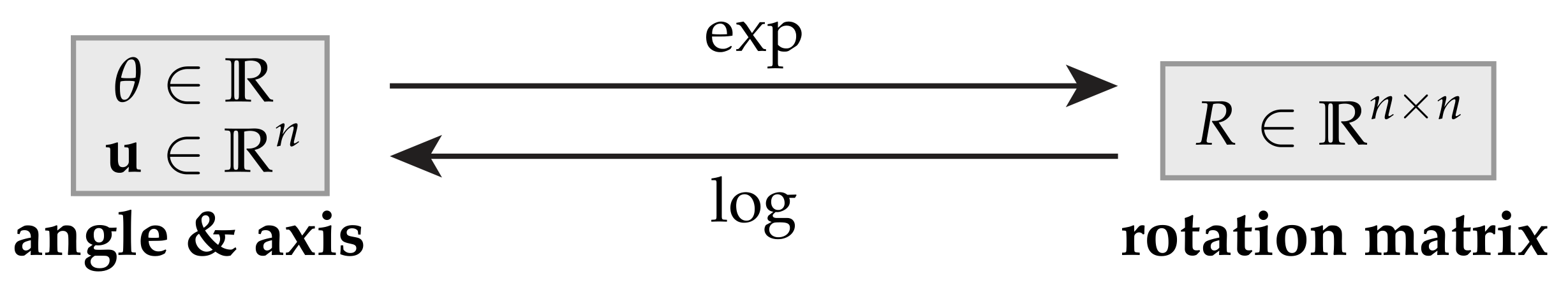
The Exponential and Logarithmic Maps
Ideally, we could freely convert rotations between these diverse representations based on our use case. We will always want to get a rotation matrix out at the end, so we’ll consider matrices the ‘canonical’ form. Enter the exponential map: a function that takes a different kind of rotation object and gives us back an equivalent rotation matrix. The corresponding logarithmic map takes a rotation matrix and gives us back a rotation object. How these maps relate to the scalar exp and log functions will hopefully become clear later on.
Below, we’ll define an exp and log map translating between rotation matrices and axis/angle vectors. But first, to build up intuition, let us consider how rotations work in two dimensions.
Axis/Angle in 2D
In 2D, there’s only one axis to rotate around: the one pointing out of the plane. Hence, our ‘axis/angle’ rotations can be represented by just $$\theta$$.
Given a 2D point $$\mathbf{p}$$, how can we rotate $$\mathbf{p}$$ by $$\theta$$? One way to visualize the transformation is by forming a coordinate frame in which the output is easy to describe. Consider $$\mathbf{p}$$ and its quarter ($$90^\circ$$) rotation $$\mathcal{J}\mathbf{p}$$:

Using a bit of trigonometry, we can describe the rotated $$\mathbf{p}_\theta$$ in two components:
But, what actually are $$\mathcal{I}$$ and $$\mathcal{J}$$? The former should take a 2D vector and return it unchanged: it’s the 2x2 identity matrix. The latter should be similar, but swap and negate the two components:
Just to make sure we got $$\mathcal{J}$$ right, let’s check what happens if we apply it twice (via $$\mathcal{J}^2$$):
We got $$\mathcal{J}^2 = -\mathcal{I}$$, which is a 180-degree rotation. So, $$\mathcal{J}$$ indeed represents 90-degree rotation.
Now, what does our transform look like?
That’s the standard 2D rotation matrix. What a coincidence!
Complex Rotations
If you’re familiar with complex numbers, you might notice that our first transform formula feels eerily similar to Euler’s formula, $$e^{ix} = \cos x + i\sin x$$:

Where $$i$$ and $$\mathcal{J}$$ both play the role of a quarter turn. We can see that in complex arithmetic, multiplying by $$i$$ in fact has that effect:
So, there must be some connection to the exponential function here.
The 2D Exponential Map
Recall the definition of the exponential function (or equivalently, its Taylor series):
Using Euler’s formula, $$e^{i\theta}$$ gave us a complex number representing a 2D rotation by $$\theta$$. Can we do the same with $$e^{\theta\mathcal{J}}$$? If we plug a matrix into the above definition, the arithmetic still works out: 2x2 matrices certainly support multiplication, addition, and scaling. (More on matrix exponentiation here.)
Let $$\theta\mathcal{J} = A$$ and plug it in:
Let’s pull out the first four terms to inspect further:
These entries look familiar. Recall the Taylor series that describe the functions $$\sin$$ and $$\cos$$:
If we write out all the terms of $$e^A$$, we’ll recover the expansions of $$\sin\theta$$ and $$\cos\theta$$! Therefore:
We’ve determined that the exponential function $$e^{\theta\mathcal{J}}$$ converts our angle $$\theta$$ into a corresponding 2D rotation matrix. In fact, we’ve proved a version of Euler’s formula with 2x2 matrices instead of complex numbers:
The 2D Logarithmic Map
The logarithmic map should naturally be the inverse of the exponential:
So, given $$R$$, how can we recover $$\theta\mathcal{J}$$?
Note that in general, our exponential map is not injective. Clearly, $$\exp(\theta\mathcal{J}) = \exp((\theta + 2\pi)\mathcal{J})$$, since adding an extra full turn will always give us back the same rotation matrix. Therefore, our logarithmic map can’t be surjective—we’ll define it as returning the smallest angle $$\theta\mathcal{J}$$ corresponding to the given rotation matrix. Using $$\text{atan2}$$ implements this definition.
Interpolation
Consider two 2D rotation angles $$\theta_0$$ and $$\theta_1$$. The most obvious way to interpolate between these two rotations is to interpolate the angles and create the corresponding rotation matrix. This scheme is essentially a 2D version of axis-angle interpolation.
However, if $$\theta_0$$ and $$\theta_1$$ are separated by more than $$\pi$$, this expression will take the long way around: it’s not aware that angles are cyclic.
| $$ \theta_0 = 0\ \ $$ | $$ \theta(0.00) = 0.00\ \ $$ | $$ \theta_1 = 4.71 $$ |
Instead, let’s devise an interpolation scheme based on our exp/log maps. Since we know the two rotation matrices $$R_0$$, $$R_1$$, we can express the rotation that takes us directly from the initial pose to the final pose: $$R_1R_0^{-1}$$, i.e. first undo $$R_0$$, then apply $$R_1$$.
Using our logarithmic map, we can obtain the smallest angle that rotates from $$R_0$$ to $$R_1$$: $$\log(R_1R_0^{-1})$$. Since $$\log$$ gives us an axis-angle rotation, we can simply scale the result by $$t$$ to perform interpolation. After scaling, we can use our exponential map to get back a rotation matrix. This matrix represents a rotation $$t$$ of the way from $$R_0$$ to $$R_1$$.
Hence, our final parametric rotation matrix is $$R(t) = \exp(t\log(R_1R_0^{-1})))R_0$$.
| $$ R_0 = \begin{bmatrix}1&0\\0&1\end{bmatrix} $$ | $$ R(0.00) = \begin{bmatrix}\phantom{-}1.00&\phantom{-}0.00\\\phantom{-}0.00&\phantom{-}1.00\end{bmatrix} $$ | $$ R_1 = \begin{bmatrix}0&-1\\1&0\end{bmatrix} $$ |
Using exp/log for interpolation might seem like overkill for 2D—we could instead just check how far apart the angles are. But below, we’ll see how this interpolation scheme generalizes—without modification—to 3D, and in fact any number of dimensions.
Axis/Angle in 3D
We’re finally ready to derive an exponential and logarithmic map for 3D rotations. In 2D, our map arose from exponentiating $$\theta\mathcal{J}$$, i.e. $$\theta$$ times a matrix representing a counter-clockwise quarter turn about the axis of rotation. We will be able to do the same in 3D—but what transformation encodes a quarter turn about a 3D unit vector $$\mathbf{u}$$?
The cross product $$\mathbf{u}\times\mathbf{p}$$ is typically defined as a vector normal to the plane containing both $$\mathbf{u}$$ and $$\mathbf{p}$$. However, we could also interpret $$\mathbf{u}\times\mathbf{p}$$ as a quarter turn of the projection of $$\mathbf{p}$$ into the plane with normal $$\mathbf{u}$$, which we will call $$\mathbf{p}_\perp$$:

So, if we can compute the quarter rotation of $$\mathbf{p}_\perp$$, it should be simple to recover the quarter rotation of $$\mathbf{p}$$. Of course, $$\mathbf{p}=\mathbf{p}_\perp+\mathbf{p}_\parallel$$, so we’ll just have to add back the parallel part $$\mathbf{p}_\parallel$$. This is correct because a rotation about $$\mathbf{u}$$ preserves $$\mathbf{p}_\parallel$$:

However, “$$\mathbf{u} \times$$” is not a mathematical object we can work with. Instead, we can devise a matrix $$\mathbf{\hat{u}}$$ that when multiplied with a a vector $$\mathbf{p}$$, outputs the same result as $$\mathbf{u} \times \mathbf{p}$$:
We can see that $$\mathbf{\hat{u}}^T = -\mathbf{\hat{u}}$$, so $$\mathbf{\hat{u}}$$ is a skew-symmetric matrix. (i.e. it has zeros along the diagonal, and the two halves are equal but negated.) Note that in the 2D case, our quarter turn $$\mathcal{J}$$ was also skew-symmetric, and sneakily represented the 2D cross product! We must be on the right track.
The reason we want to use axis/angle rotations in the first place is because they form a vector space. So, let’s make sure our translation to skew-symmetric matrices maintains that property. Given two skew-symmetric matrices $$A_1$$ and $$A_2$$:
Their sum is also a skew-symmetric matrix. Similarly:
Scalar multiplication also maintains skew-symmetry. The other vector space properties follow from the usual definition of matrix addition.
Finally, note that $$\mathbf{u} \times (\mathbf{u} \times (\mathbf{u} \times \mathbf{p})) = -\mathbf{u} \times \mathbf{p}$$. Taking the cross product three times would rotate $$\mathbf{p}_\perp$$ three-quarter turns about $$\mathbf{u}$$, which is equivalent to a single negative-quarter turn. More generally, $$\mathbf{\hat{u}}^{k+2} = -\mathbf{\hat{u}}^k$$ for any $$k>0$$. We could prove this by writing out all the terms, but the geometric argument is easier:

The 3D Exponential Map
Given an axis/angle rotation $$\theta\mathbf{u}$$, we can make $$\theta\mathbf{\hat{u}}$$ using the above construction. What happens when we exponentiate it? Using the identity $$\mathbf{\hat{u}}^{k+2} = -\mathbf{\hat{u}}^k$$:
In the last step, we again recover the Taylor expansions of $$\sin\theta$$ and $$\cos\theta$$. Our final expression is known as Rodrigues’ formula.
This formula is already reminiscent of the 2D case: the latter two terms are building up a 2D rotation in the plane defined by $$\mathbf{u}$$. To sanity check our 3D result, let’s compute our transform for $$\theta = 0$$:
Rotating by $$\theta = 0$$ preserves $$\mathbf{p}$$, so the formula works. Then compute for $$\theta = \frac{\pi}{2}$$:
Above, we already concluded $$\mathbf{u}\times\mathbf{p} + \mathbf{p}_\parallel$$ is a quarter rotation. So, our formula is also correct at $$\theta = \frac{\pi}{2}$$. Then compute for $$\theta = \pi$$:

We end up with $$-\mathbf{p}_\perp + \mathbf{p}_\parallel$$, which is a half rotation. Hence $$\theta = \pi$$ is also correct.
So far, our formula checks out. Just to be sure, let’s prove that our 3D result is a rotation matrix, i.e. it’s orthonormal and has positive determinant. A matrix is orthonormal if $$A^TA = \mathcal{I}$$, so again using $$\mathbf{\hat{u}}^{k+2} = -\mathbf{\hat{u}}^k$$:
Therefore, $$e^{\theta\mathbf{\hat{u}}}$$ is orthonormal. We could show its determinant is positive (and therefore $$1$$) by writing out all the terms, but it suffices to argue that:
- Clearly, $$\begin{vmatrix}\exp(0\mathbf{\hat{u}})\end{vmatrix} = \begin{vmatrix}\mathcal{I}\end{vmatrix} = 1$$
- There is no $$\theta$$, $$\mathbf{\hat{u}}$$ such that $$\begin{vmatrix}\exp(\theta\mathbf{\hat{u}})\end{vmatrix} = 0$$, since $$\mathbf{\hat{u}}$$ and $$\mathbf{\hat{u}}^2$$ can never cancel out $$\mathcal{I}$$.
- $$\exp$$ is continuous with respect to $$\theta$$ and $$\mathbf{\hat{u}}$$
Therefore, $$\begin{vmatrix}\exp(0\mathbf{\hat{u}})\end{vmatrix}$$ can never become negative. That means $$\exp(\theta\mathbf{\hat{u}})$$ is a 3D rotation matrix!
The 3D Logarithmic Map
Similarly to the 2D case, the 3D exponential map is not injective, so the 3D logarithmic map will not be surjective. Instead, we will again define it to return the smallest magnitude axis-angle rotation corresponding to the given matrix. Our exponential map gave us:
We can take the trace (sum along the diagonal) of both sides:
Clearly $$\operatorname{tr}(\mathcal{I}) = 3$$, and since $$\mathbf{\hat{u}}$$ is skew-symmetric, its diagonal sum is zero. That just leaves $$\mathbf{\hat{u}}^2$$:
We can see $$\operatorname{tr}(\mathbf{\hat{u}}^2) = -2u_x^2-2u_y^2-2u_z^2 = -2|\mathbf{u}|^2 = -2$$. (We originally defined $$\mathbf{u}$$ as a unit vector.) Our final trace becomes:
That’s half of our logarithmic map. To recover $$\mathbf{\hat{u}}$$, we can antisymmetrize $$R$$. Recall $$\mathbf{\hat{u}}^T = -\mathbf{\hat{u}}$$, and that $$\mathbf{\hat{u}}^2$$ is symmetric (above).
Finally, to get $$\mathbf{u}$$, we can pull out the entries of $$\mathbf{\hat{u}}$$, which we just derived:
We now have our full 3D logarithmic map!
Interpolation
Now equipped with our 3D exp and log maps, we can use them for interpolation. The exact same formula as the 2D case still applies:
| $$ R_0 = \begin{bmatrix}1&0&0\\0&1&0\\0&0&1\end{bmatrix} $$ | $$ R(0.00) = \begin{bmatrix}\phantom{-}1.00&\phantom{-}0.00&\phantom{-}0.00\\\phantom{-}0.00&\phantom{-}1.00&\phantom{-}0.00\\\phantom{-}0.00&\phantom{-}0.00&\phantom{-}1.00\end{bmatrix} $$ | $$ R_1 = \begin{bmatrix}-0.42&-0.59&-0.69\\0.51&-0.79&0.36\\-0.75&-0.20&0.63\end{bmatrix} $$ |
Our interpolation scheme produces all the nice properties of axis/angle rotations—and chooses the shortest path every time. This wouldn’t look so smooth with Euler angles!
Averaging Rotations
However, we would have gotten an equally good interpolation scheme by just using quaternions instead of messing about with all this matrix math. Let’s consider something interesting we can only easily do with axis/angle rotations: averaging a set of rotation matrices.
The most straightforward method is to convert each matrix into an axis/angle rotation, average the resulting vectors, and convert back. That is certainly a valid strategy, but the resulting behavior won’t be very intuitive:
In particular, summing axis-angle vectors can result in “catastrophic cancellation.” An extreme example is averaging $$\begin{bmatrix}\pi&0&0\end{bmatrix}$$ and $$\begin{bmatrix}-\pi&0&0\end{bmatrix}$$, resulting in zero—which is clearly not representative of the two equivalent rotations.
To find an alternative, let’s first consider a slightly unconventional way of averaging points in the plane. The average of a set of points is the point that minimizes total squared distance to all others. Hence, there’s an optimization-based algorithm for finding it. Given $$x_0, \dots, x_n$$, we can iterate the following procedure:
- Pick an initial guess $$\bar{x} \in \mathbb{R}^2$$ (can be one of the points).
- Repeat:
- For each point, get its translation from the guess: $$\mathbf{u}_i \leftarrow x_i - \bar{x}$$
- Average the vectors: $$\mathbf{u} \leftarrow \frac{1}{n} \sum_{i=1}^n \mathbf{u}_i$$
- Step toward the average direction: $$\bar{x} \leftarrow \bar{x} + \tau\mathbf{u}$$
- while $$|\mathbf{u}| > \epsilon$$.

As we run this procedure, $$\bar{x}$$ will converge to the average point. Of course, we could have just averaged the points directly, but we’ll be able to translate this idea to the rotational case rather nicely.
Our logarithmic map lets us convert rotation matrices to axis axis/angle rotations, which are themselves just 3D points. So, what if we use the point averaging algorithm on rotations $$R_0, \dots, R_n$$?
- Pick an initial guess $$\bar{R} \in \mathbb{R}^{3\times3}$$ (can be $$\mathcal{I}$$).
- Repeat:
- For each matrix, get its axis/angle rotation from the guess: $$\mathbf{u}_i \leftarrow \log(R_i\bar{R}^{-1})$$
- Average the vectors: $$\mathbf{u} \leftarrow \frac{1}{n} \sum_{i=1}^n \mathbf{u}_i$$
- Step toward the average rotation: $$\bar{R} \leftarrow \exp(\tau\mathbf{u})\bar{R}$$
- while $$|\mathbf{u}| > \epsilon$$.
The result of this algorithm is formally known as the Karcher mean. Just like how the average point minimizes total squared distance from all other points, the Karcher mean is a rotation that minimizes squared angular distance from all other rotations. Therefore, it won’t be subject to catastrophic cancellation—we’ll always end up with a non-zero in-between rotation.
Try comparing the two averaging algorithms—randomizing will keep them in sync. While the results are often similar, the Karcher mean exhibits more consistent behavior.
Quaternions (Again)
Warning: section assumes knowledge of quaternions
Okay, I couldn’t resist talking about quaternions at least a little bit, given how closely they’re related to axis/angle rotations. Just like how complex exponentiation turned out to be equivalent to (skew-symmetric) 2D matrix exponentiation, quaternion exponentiation is equivalent to (skew-symmetric) 3D matrix exponentiation.
In 2D, an axis/angle rotation was simply $$\theta$$. We created a pure-imaginary complex number $$i\theta$$ and exponentiated it:
We got back a complex number that when multiplied with a point, rotates it by $$\theta$$. It’s always the case that $$|\cos\theta + i\sin\theta| = 1$$, so 2D rotations can be represented as unit-norm complex numbers.
In 3D, an axis/angle rotation is a vector $$\mathbf{u}$$ such that $$|\mathbf{u}| = \theta$$. What happens if we create a pure-imaginary quaternion $$\mathbf{q} = u_x\mathbf{i} + u_y\mathbf{j} + u_z\mathbf{k}$$ and exponentiate it, too?
To make evaluating $$e^\mathbf{q}$$ easier, first derive the following using the quaternion multiplication rules:
Which is highly reminiscent of the skew-symmetric matrix identity used above. Therefore…
Our result looks almost exactly like the 2D case, just with three imaginary axes instead of one. In 2D, our axis/angle rotation became a unit-norm complex number. In 3D, it became a unit-norm quaternion. Now we can use this quaternion to rotate 3D points! Pretty cool, right?
One advantage of using quaternions is how easy the exponential map is to compute—if you don’t need a rotation matrix, it’s a good option. The quaternion logarithmic map is similarly simple:
Finally, note that the way to rotate a point $$\mathbf{p}$$ by a quaternion $$\mathbf{q}$$ is by evaluating the conjugation $$\mathbf{q}\mathbf{p}\mathbf{q}^{-1}$$, where $$\mathbf{p} = p_x\mathbf{i} + p_y\mathbf{j} + p_z\mathbf{k}$$ is another pure-imaginary quaternion representing our point. The conjugation technically rotates the point by $$2\theta$$ about $$\mathbf{u}$$, but that’s easily accounted for by making $$|\mathbf{u}| = \frac{\theta}{2}$$ in the beginning.
Further Reading
Made it this far? Well, there’s even more to learn about rotations.
Learn about quaternions here, and why geometric algebra is more intuitive here.
Beyond understanding the four representations covered here (plus geometric algebra), it can be enlightening to learn about the algebraic structure underlying all 3D rotations: the group $$SO(3)$$. I found this video to be a great resource: it explains $$SO(3)$$ both intuitively and visually, demonstrating how it relates it to the group $$SU(2)$$ as well as why quaternions and axis/angle rotations double-cover 3D rotation matrices.
The wikipedia page on SO(3) is also informative, though very math heavy. It touches on connections with axis/angle rotations, topology, $$SU(2)$$, quaternions, and Lie algebra. It turns out the vector space of skew-symmetric matrices we derived above makes up $$\mathfrak{so}(3)$$, the Lie algebra that corresponds to $$SO(3)$$.